Estimating the the drag coefficient’s curve basing on data from a WHPSC run

Assuming certain atmospheric conditions, simulations help understanding which power input is necessary to reach a certain speed. As the objective is to break the world record in speed at the World Human Powered Vehicles Challenge (WHPSC) in Nevada, gaining knowledge about the bike’s performance is fundamental. Moreover, being able to simulate a run before actually getting to the race location allows estimating the potential of a bike.

These simulations use an energy balance equation. Given the speed v(j) at the j-th time step, it’s obtained the speed at the next time step by solving the equation for v(j+1). Within the equation there are the various energy contributes: kinetic energy (Ec), positive contributes (power input and the negative slope) and negative contributes (rolling- and drag resistance). The latter are respectively given by:

E_r=m*g*C_r dl
E_d=1/2*rho*A*C_d*v^2 dl

where:

• m: mass of the vehicle,
• g: gravitational acceleration,
• dl: distance covered in the time interval,
• rho: air density,
• A: frontal area,
• v: vehicle speed [m/s],
• C_r: coefficient of rolling resistance,
• C_d: coefficient of drag resistance.

Both coefficients depend on speed. If aree considered the other terms in the equation to be “reasonably correct”, the more precise the coefficients are determined, the more accurate is the result of the run simulated. Values for C_r’s curve are obtained on our testing facility, while C_d’s profile relies on values obtained in a CFD simulation.

Therefore, it’s important to assess the accuracy of the CFD simulation (measured on the outcome; i.e. the simulated speed). Moreover, as it is performed under static conditions (vehicle not moving, wind coming at different speeds), it leaves out the interaction between vehicle and rider.

A four-step procedure is identified todetermine a ”realistic”profile basing on data from a WHPSC run. It has been used a non-dimensional random variable z

z(j) = error(j)/Ec(j+1) 

where:
error(j): error in the j-th energy balance equation,
Ec(j+1) : kinetic energy at the end of the j-th time interval

Thereon, it’s first apply a low-pass filter and consider an average deviation in the energy balance equation. Secondly, it’s determined the drag coefficient by solving the energy balance equation for C_d and average the obtained value. Finally, we sample C_d’s vector containing values at different speeds, keeping a reasonable number (about 10), one every about 15/ 20 km/h.

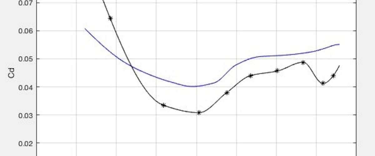
The obtained graphs are shown here below. They differ slightly for high speeds (around 35 m/s), being quite similar for the rest. Note that the scale of the axis has been altered.

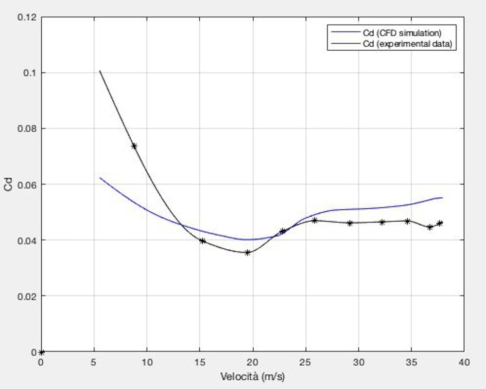
Drag coefficient (BM 19 Thursday PM ride)

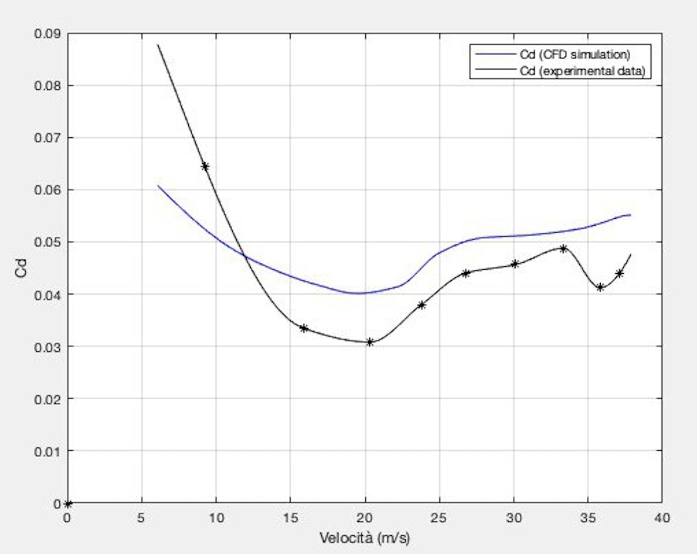
Drag coefficient (BM 19 Friday PM ride)